Learn · Two
Quantifying oscillations in natural images and sounds
A coastline is not a signal. It is light arriving at a sensor, indexed by two spatial dimensions and one temporal one, and none of that can be set beside a heartbeat until it has become a single number that changes over time.
That reduction is a choice, and there are many honest ways to make it. This page walks through the main ones and shows what each keeps and what each throws away. Some figures use real footage with the measures computed live from its pixels; others use synthesised scenes, because the only way to prove a method works is to hand it data whose answer you already know.
Part one
A scene is not a signal
Three dimensions have to become one. What that costs, and why the answer depends on how much of the frame each number is asked to stand for.
The problem
How much of the frame should one number mean?
Every measure on this page begins by collapsing a frame to fewer numbers than it contains. The question is how far to collapse it. Average the whole image and you get one value that is cheap, stable and often nearly blind. Keep every pixel separately and you get a map that is precise, expensive and fragile. Between them sits a grid of patches, which is where a great deal of practical work actually lives.
Four ways to turn a moving scene into one number
Blind to · anything the reduction averages away. A whole-image mean cannot see where in the frame something happened, and by construction it barely sees a travelling wave at all.
In one sentence
The spatial scale is not a technical setting. It decides which questions the rest of the analysis is even able to ask.
The same thing on real video
Three seas, one set of measures
Synthetic scenes are useful because you know the answer in advance. Real footage is useful because it does not cooperate. Below are three clips of moving water, with the measures computed in the browser frame by frame as the video plays.
Switch between the clips with the same view selected and watch the numbers move. A long breaking swell and a short choppy surface are obviously different to look at, and the point is that they are also different in a way a measure can report without anybody describing the scene to it.
Wave clips, measured as they play
Source
Press play. Nothing is computed until the clip runs.
Traces, building as it plays
In one sentence
These measures never learn what water is. They report how brightness is distributed and how it changes, and the difference between a swell and a chop falls out of that on its own.
Browser arithmetic is necessarily crude. The traces below come from the project’s analysis pipeline instead, which uses dense optical flow and proper complexity estimators. Same footage, better instruments.
Optical flow, texture and complexity
Magnitude · how much motion
0.000 to 0.162
Curl · how much rotation
0.000 to 0.016
Direction entropy · how scattered
0.000 to 6.405
- Magnitude · how much motion
- Curl · how much rotation
- Direction entropy · how scattered
In one sentence
Direction entropy is the one to notice. Two clips can carry identical average motion and still be told apart by whether the frame agrees about which way it is going.
Part two
Reading rhythm out of a scene
Three ways to get a frequency out of moving pixels: sample one line and read time as an image, measure how power spreads across scales, or decompose the motion into oscillating patterns.
The oceanographer's trick
Timestacks: one column, read as an image of time
The question it asks
How long does a wave take to pass a fixed line?
Take a single column of pixels and record it at every frame, then lay those columns side by side. Space runs down the result and time runs across it, so a wave moving past the column draws a diagonal stripe, and the spacing between stripes is the wave period. It is an unreasonably economical method: one line out of a whole scene, and the number falls out.
Timestack · one column, stacked over time
Blind to · anything that does not cross the sampled line coherently. Short-crested chop never builds a stripe, which is a weakness if the chop is what you care about and a strength if it is not.
In one sentence
Discarding almost the entire frame can make a measurement more robust rather than less. What matters is whether what you kept carries the structure you are asking about.
Structure across scales
Scale-free, in space and in time
The question it asks
Is any scale privileged, or is structure spread evenly across all of them?
Natural scenes have a statistical signature that has nothing to do with what is in them. Take the two-dimensional spectrum of almost any photograph of a landscape and power falls off as roughly one over spatial frequency squared, which is to say structure exists at every size with none dominating. The same is true along the time axis of a great many natural sounds.
Scale-free structure in an image and in a sound
Blind to · arrangement. A slope says how power is spread across scales and nothing about where anything is, so a landscape and a shuffled version of that landscape can score identically.
In one sentence
An image and a sound are the same kind of object one axis apart, which is why the same handful of operations serves both.
Decomposition
A scene as a few oscillating patterns
The question it asks
Can the motion be written as a small number of fixed patterns taking turns?
Often it can. Rather than a frequency per pixel or one number for the whole frame, look for the handful of spatial patterns whose brightnesses oscillate, and describe the clip as their sum. A long video becomes a few images and a few traces, with very little worth worrying about lost.
Modal decomposition · a scene as a few oscillating patterns
Blind to · anything that is not a sum of steady patterns. A scene whose structure changes partway through needs the decomposition refitted in a sliding window, or it will average the two regimes into something that describes neither.
In one sentence
Modes arrive in pairs because a standing pattern cannot travel. Reading a decomposition means reading the pairs, not the individual modes.
Those were synthesised, so the answer was known in advance. Below are modes decomposed from footage, drawn as reliefs that oscillate at the frequencies the pipeline found for them.
Spatial modes, breathing at their own frequencies
Mode 1
0.18 Hz · 100%
Mode 2
0.29 Hz · 91%
Mode 3
0.09 Hz · 86%
Mode 4
0.34 Hz · 68%
Putting it together
Four seas, told apart by numbers alone
The question it asks
Can measures that know nothing about water sort these clips the way a person would?
Four clips of moving water, each run through the whole pipeline. None of these measures has any concept of a wave, a horizon or foam. They report how brightness is arranged, how it moves and how regular that movement is, and that turns out to be enough to separate an ordered swell from a broken sea.
Four clips, four sets of numbers
Pixel synchrony · how much of the frame oscillates together
Clip one
broken, fast, scattered
0.141
Frequency per pixel
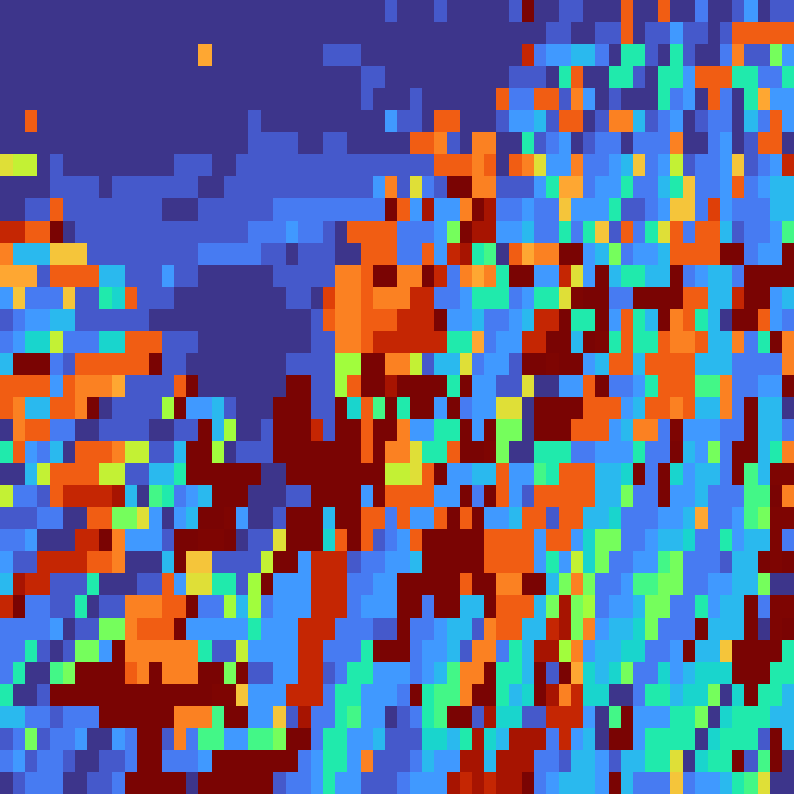
Leading pattern

Modal energy
- Wave frequency
- 1.50 Hz
- Pixel coherence
- 0.940
Clip two
long swell, moderately organised
0.410
Frequency per pixel
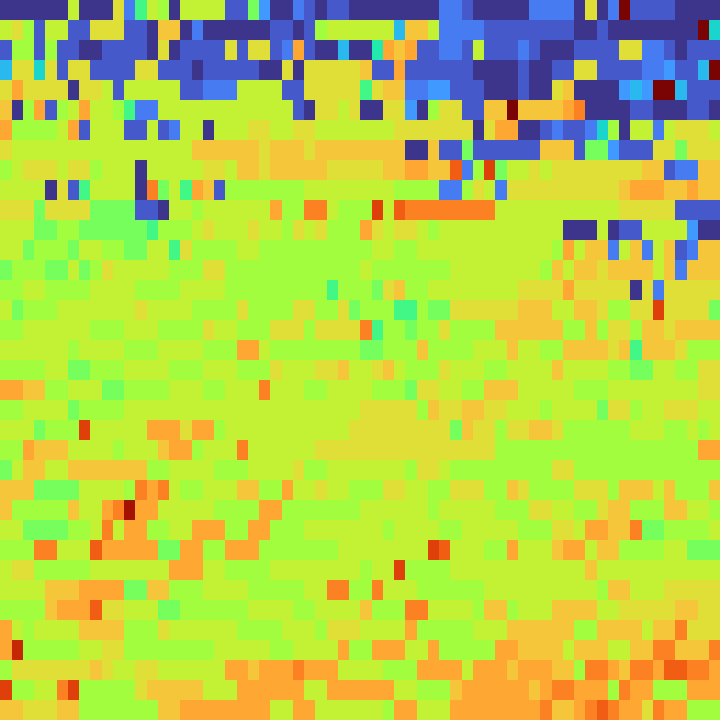
Leading pattern

Modal energy
- Wave frequency
- 0.12 Hz
- Pixel coherence
- 0.976
Clip three
the most organised of the four
0.553
Frequency per pixel
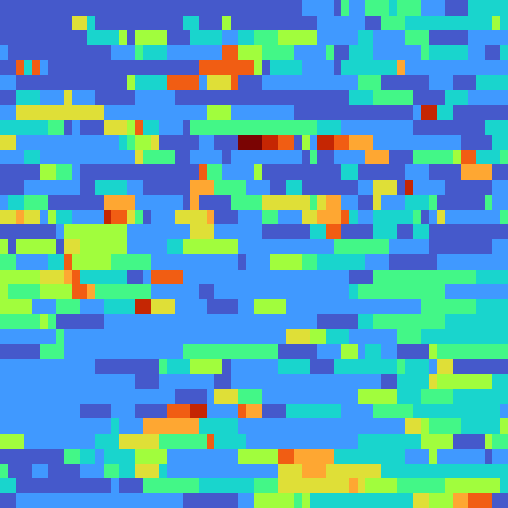
Leading pattern

Modal energy
- Wave frequency
- 0.12 Hz
- Pixel coherence
- 0.988
Clip four
broken and fast, like clip one
0.140
Frequency per pixel
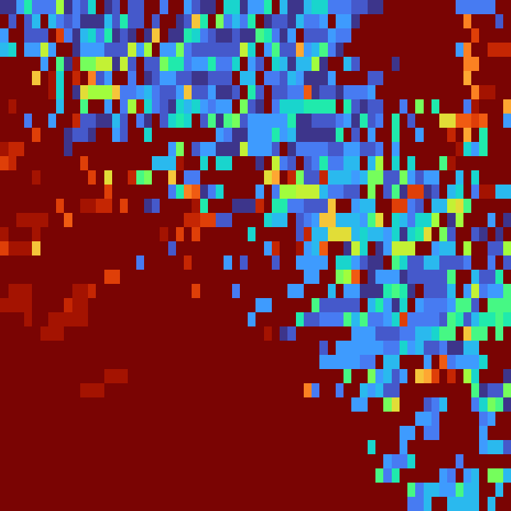
Leading pattern

Modal energy
- Wave frequency
- 1.38 Hz
- Pixel coherence
- 0.907
Blind to · meaning. These numbers separate the clips reliably and say nothing whatever about which sea a person would rather sit beside, which is a different question and needs a different instrument.
In one sentence
A measurement that agrees with your eye on cases you can check is a measurement you can begin to trust on cases you cannot.
Part three
The whole space
Two decisions, crossed. One of them is new; the other you have met before.
Zooming out
Spatial scale crossed with feature family
Every extractor on this page is a choice of how much of the frame one number stands for, crossed with a choice of what about it to measure. The first decision is particular to images. The second is not: the columns below are the same three feature families that organise every coupling method, because once a scene has been reduced to a trace it stops mattering that it came from a camera.
The video matrix · spatial scale × feature family
Rawthe values themselves | Oscillatoryrhythm and spatial frequency | Complexityroughness and regularity | |
|---|---|---|---|
Whole imageone number per frame | |||
Per patcha coarse grid, one number per tile | |||
Per pixelevery pixel its own time series |
Raw · whole image
luminance · frame difference · optical flow. The cheapest tier and the most used. Optical flow is the interesting member: as well as a magnitude it yields curl, divergence and the entropy of flow direction, so a scene where everything moves the same way is distinguishable from one where motion is scattered even when the total is identical.
In one sentence
A video is not a special kind of data. It is an expensive way to arrive at the same one-dimensional traces everything else produces, and the expense buys you a choice about spatial scale that a microphone never offers.
Where a figure synthesises a scene it also checks itself: the spectral slope recovers the value it was given to within a hundredth, and the timestack recovers a swell frequency to within half a bin even under heavy chop. The figures that sample video reduce frames on a small grid in the browser, which is coarser than the offline pipeline and behaves the same way. Still to be written: optical flow in its own right, per-pixel frequency maps, and what changes when the camera is moving too.